The eigenproblem solver in my master's thesis used SuperLU, a direct solver for the solution of systems of linear equations (SLE) $Ax = b$. For the largest test problems, the eigensolver ran out of memory when decomposing the matrix $A$ which is why I replaced SuperLU with direct substructuring in an attempt to reduce memory consumption. For this blog post, I measured set-up time, solve time, and memory consumption of SuperLU and direct substructuring with real symmetric positive definite real-world matrices for SLEs with a variable number of right-hand sides, I will highlight that SuperLU was deployed with a suboptimal parameter choice, and why the memory consumption of the decomposition of $A$ is the wrong objective function when you want to avoid running out of memory.

Introduction

For my master's thesis, I implemented a solver for large, sparse generalized eigenvalue problems that used SuperLU to solve SLEs $A x = b$, where $A \in \mathbb{C}^{n,n}$ is large, sparse, and Hermitian positive definite (HPD) or real symmetric positive definite. SuperLU is a direct solver for such SLEs but depending on the structure of the non-zero matrix entries, there may be so much fill-in that the solver runs out of memory when attempting to factorize $A$ and this happened for the largest test problems in my master's thesis. Without carefully measuring the memory consumption, I replaced SuperLU with direct substructuring.

Direct substructuring is a recursive method for solving SLEs $Ax = b$.  Partition
$$A = \begin{pmatrix} A_{11} & A_{12} \\ A_{21} & A_{22} \end{pmatrix}, x = \begin{pmatrix} x_1 \\ x_2 \end{pmatrix}, b = \begin{pmatrix} b_1 \\ b_2 \end{pmatrix}$$
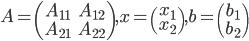
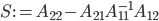
conformally and let $S$ be the Schur complement of $A_{11}$ in $A$:
$$S := A_{22} - A_{21} A_{11}^{-1} A_{12}$$
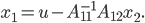
Then we can compute $x$ as follows: solve $A_{11} u = b_1$ and calculate 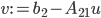$v := b_2 - A_{21} u$. Then
$$x_2 = S^{-1} v.$$
Finally,
$$x_1 = u - A_{11}^{-1} A_{12} x_2.$$
Our aim is to solve SLEs $Ax = b$ and so far, I did not explain how to solve SLEs $A_{11} y_1 = c_1$. We could solve this SLE directly with a dense or a sparse solver or we can apply the idea from above again, i.e., we partition $A_{11}$ into a $2 \times 2$ block matrix, partition $x_1$ and $b_1$ conformally, and solve $A_{11} x_1 = b_1$. This recursive approach yields a method that is called direct substructuring and it belongs to the class of domain decomposition methods. Usually, direct substructuring is used in conjunction with Krylov subspace methods; the SLE solver MUMPS is an exception to this rule. See the paper Iterative versus direct parallel substructuring methods in semiconductor device modeling for a comparison of these approaches.

Observe for direct substructuring, we only need to store the results of the factorization of the Schur complements, e.g., the matrices $L$ and $U$ of the LU decomposition of $S$ so the memory consumption of the factorization of $A$ is a function of the dimension of $A_{22}$. Furthermore, we can quickly minimize the dimension of the block $A_{22}$ with the aid of nested dissection orderings, a method based on minimal vertex separators in graph theory. Thus, it is possible to use direct substructuring in practice.

Before presenting the results of the numerical experiments, I elaborate on the suboptimal parameter choice for SuperLU and afterwards, I explain why using direct substructuring was ill-advised.

SuperLU and Hermitian Positive Definite Matrices

SuperLU is a sparse direct solver meaning it tries to find permutation matrices $P$ and $Q$ as well as triangular matrices $L$ and $U$ with minimal fill-in such that $P A Q = LU$. When selecting permutation matrices, SuperLU considers fill-in and the modulus of the pivot to ensure numerical stability; $P$ is determined from partial pivoting and $Q$ is chosen independently from $P$ in order to minimize fill-in (see Section 2.5 of the SuperLU User's Guide). SuperLU uses threshold pivoting meaning SuperLU attempts to use the diagonal entry $a_{ii}$ as pivot unless
$$\lvert a_{ii} \rvert < c \max_{j < i} \lvert a_{ij} \rvert,$$
where $c \geq 0$ is a small, user-provided constant. Consequently, for sufficiently well-conditioned HPD matrices, SuperLU will use $P = Q$ and compute a Cholesky decomposition such that $P^* A P = L L^*$, approximately halving the memory consumption in comparison to an LU decomposition. For badly conditioned or indefinite matrices, SuperLU will thus destroy hermiticity as soon as a diagonal element violates the admission criterion for pivoting elements above and compute an LU decomposition.

For HPD matrices small pivots $\lvert a_{ii} \rvert$ do not hurt numerical stability and in my thesis, I used only HPD matrices. For large matrices, SuperLU was often computing LU instead of Cholesky decompositions and while this behavior is completely reasonable, it was also unnecessary and it can be avoided by setting $c := 0$ thereby forcing SuperLU to compute Cholesky factorizations.

Optimizing for the Wrong Objective Function

Given an SLE $A x = b$ and a suitable factorization of $A$, a direct solver can overwrite $b$ with $x$ such that no temporary storage is needed. Hence as long as there is sufficient memory for storing the factorization of $A$ and the right-hand sides $b$, we can solve SLEs.

Let us reconsider solving an SLE with direct substructuring. We need to

• solve $A_{11} u = b_1$,
• calculate $v := b_2 - A_{21} u$,
• solve $S x_2 = v$, and
• compute $x_1 = u - A_{11}^{-1} A_{12} x_2$.

Let $w := A_{11}^{-1} A_{12}$. Observe when computing $x_1$ in the last step, we need to store $u$ and $w$ simultaneously. Assuming we overwrite the memory location originally occupied by $b_1$ with $u$, we still need additional memory to store $w$. Thus, direct substructuring requires additional memory during a solve because we need to store the factorized Schur complements as well as $w$. That is, the maximum memory consumption of direct substructuring may be considerably larger than the amount of memory required only for storing the Schur complements. The sparse solver in my thesis was supposed to work with large matrices (ca. $10^5 \times 10^5$) so even if the block $A_{22}$ is small in dimension such that $A_{12}$ has only few columns, storing $w$ requires large amounts of memory, e.g., let $m \in \mathbb{N}$ such that $A_{22} \in \mathbb{C}^{m,m}$, let $m = 200$ and let $n = 100,000$. With double precision floats (8 bytes), $w$ requires
$$8\text{B} \cdot n (n-m) \approx 153\text{MiB}$$
of storage. For comparison, storing the $m \times m$ matrix $S$ consumes 0.3MiB while the 2,455,670 non-zeros of the test matrix s3dkq4m2 (see the section with the numerical experiments) with dimension 90,449 require 18.7MiB of memory, and the sparse Cholesky factorization of s3dkq4m2 computed by SuperLU occupies 761MiB. Keep in mind that direct substructuring is a recursive method, i.e., we have to store a matrix $w$ at every level of recursion.

If we want to avoid running out of memory, then we have to reduce the maximum memory usage. When I decided to replace SuperLU with direct substructuring, I attempted to reduce the memory required for storing the matrix factorization.  With SuperLU, maximum memory consumption and memory required for storing the matrix factorization are the same but not for direct substructuring. In fact, the maximum memory consumption is often magnitudes larger than the storage required for the factors of the Schur complements.

Numerical Experiments

I measured the following quantities:

• fill-in,
• maximum memory consumption,
• the time needed to factorize $A$, and
• the time needed to solve SLEs with 256, 512, 1024, and 2048 right-hand sides (RHS).

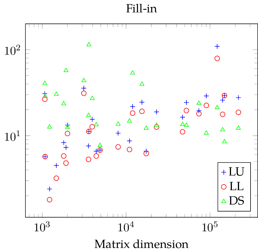
In the plots, LU signifies SuperLU with the default parameters, LL stands for SuperLU with parameters chosen to exploit hermiticity ($LL$ is an allusion to the Cholesky decomposition $A = LL^*$, see the section on SuperLU and HPD matrices), and DS means direct substructuring. The set of 27 test matrices consists of all real symmetric positive definite Harwell-Boeing BCS structural engineering matrices, as well as

• gyro_k, gyro_m,
• vanbody,
• ct20stif,
• s3dkq4m2,
• oilpan,
• ship_003,
• bmw7st_1,
• bmwcra_1, and
• pwtk.

These matrices can be found at the University of Florida Sparse Matrix Collection. The smallest matrix has dimension 1074, the largest matrix has dimension 217,918, the median is 6458, and the arithmetic mean is 37,566. For the timing tests, I measured wall-clock time and CPU time and both timers have a resolution of 0.1 seconds. The computer used for the tests has an AMD Athlon II X2 270 CPU and 8GB RAM. Direct substructuring was implemented in Python with SciPy 0.17.1 and NumPy 1.10.4 using Intel MKL 11.3. SuperLU ships with SciPy. The right-hand sides vectors $b$ are random vectors with uniformly distributed entries in the interval $[-1, 1)$.

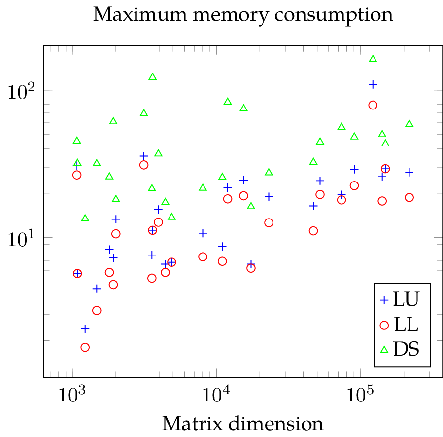
With the fill-in plot, it is easy to see that LL requires less memory than LU. For direct substructuring, the fill-in is constant except for a few outliers where the matrix $A$ is diagonal. For the smallest problems, both SuperLU variants create less fill-in but for the larger test matrices, DS is comparable to LL and sometimes better. Unfortunately, we can also gather from the plot that the fill-in seems to be a linear function of the matrix dimension $n$ with SuperLU. If we assume that the number of non-zero entries in a sparse matrix is a linear function of $n$, too, then the number of non-zero entries in the factorization must be proportional to $n^2$. When considering maxmimum memory consumption, DS is significantly worse than LL and LU.

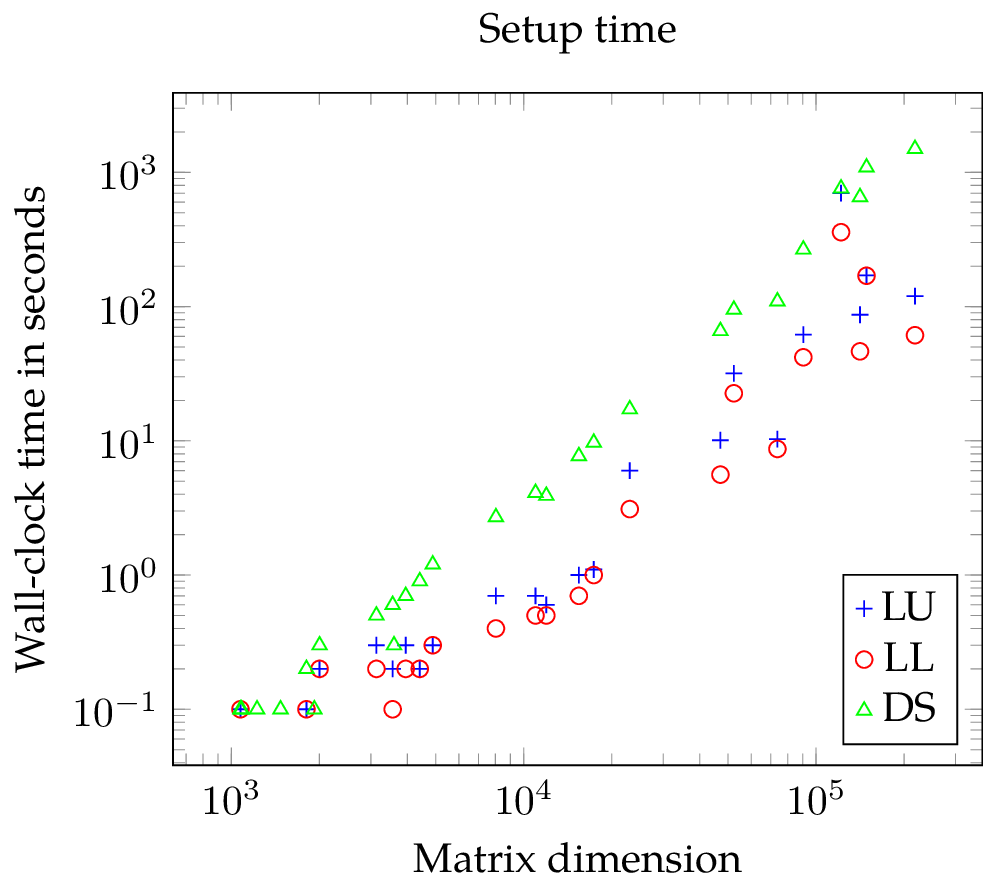
The plot showing the setup time of the solvers are unambiguous: LL needs slightly less time than LU and LL as well as LU require both significantly less time than DS (note the logarithmic scale).

Before I present the measurements for the time needed to solve the SLEs, I have to highlight a limitation of SciPy's SuperLU interface. As soon as one computed the LU or Cholesky decomposition of a matrix $A$ of an SLE $Ax = b$, there is no need for additional memory because the RHS $b$ can be overwritten directly with $x$. This is exploited by software, e.g., LAPACK as well as SuperLU. Nevertheless, SciPy's SuperLU interface stores the solution $x$ in newly allocated memory and this leaves SuperLU unable to solve seven (LU) and six SLEs (LL), respectively. For comparison, DS is unable to solve six SLEs.

The time needed to solve an SLE depends on the number of RHS, on the dimension of the matrix $A$, other properties of $A$ like node degrees. To avoid complex figures, I plotted the solve time normalized by the time needed by LL for solving an SLE with 256 RHS and the same matrix $A$ over the number of RHS and the results can be seen below. Due to the normalization, I removed all SLEs where LL was unable to solve $Ax = b$ with 256 RHS. Moreover, the plot ignores all SLEs where the solver took less than one second to compute the solution to reduce jitter caused by the timer resolution (0.1 seconds) and finally, I perturbed the $x$-coordinate of the data points to improve legibility.

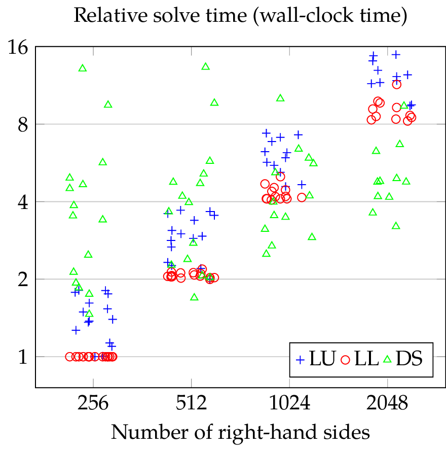
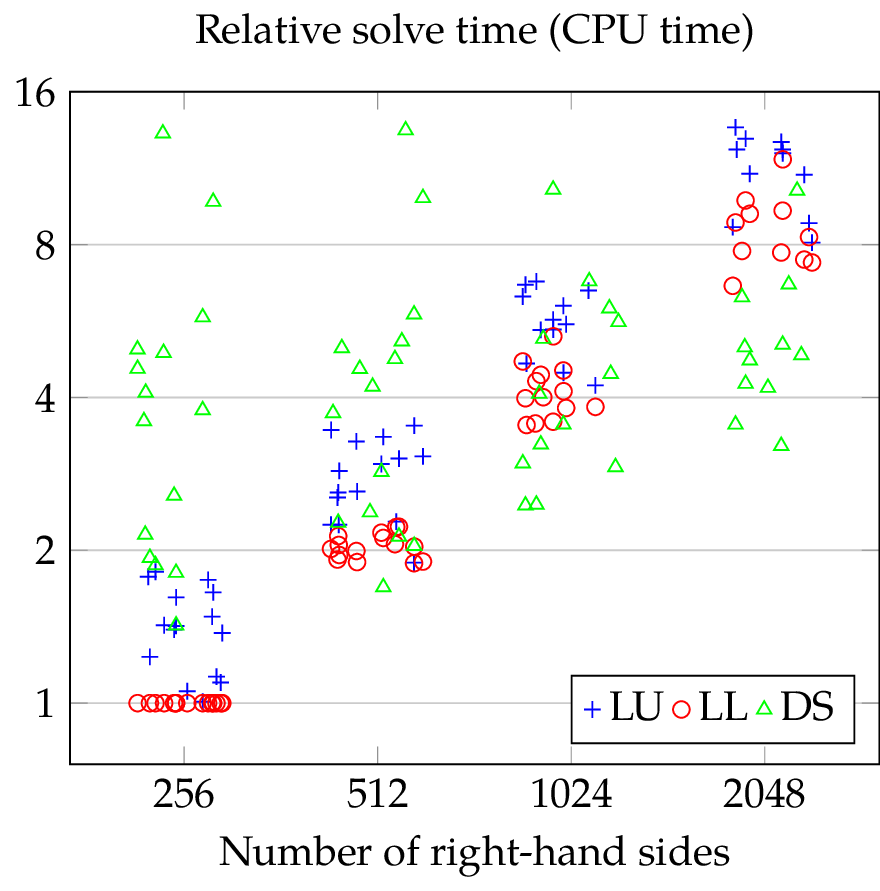
For most problems, LL is faster than LU and for both solvers, the run-time increases linearly with the number of RHS as expected (this fact is more obvious when considering CPU time). For DS, the situtation is more interesting: with 256 RHS, DS is most of the time signifcantly slower than both LL and LU but with 2048 RHS, DS is often significantly faster than both LL and LU. To explain this behavior, let us reconsider the operations performed by DS ($A$ is a $2 \times 2$ block matrix):

• solve $A_{11} u = b_1$,
• calculate $v := b_2 - A_{21} u$,
• solve $S x_2 = v$, and
• compute $x_1 = u - A_{11}^{-1} A_{12} x_2$.

Let $m$ be the number of RHS (the number of columns of $b$) and let $n_2$ be the number of columns of $A_{12}$.  In practice, $A_{22}$ will be considerably smaller than $A_{11}$ in dimension hence the majority of computational effort is required for the evaluation of $A_{11}^{-1} b_1$ and $A_{11}^{-1} A_{12} x_2$. If we evaluate the latter term as $(A_{11}^{-1} A_{12}) x_2$, then DS behaves almost as if there were $m + n_2$ RHS. For small $m$, this will clearly impact the run-time, e.g., with $m \approx n_2$, the number of RHS is effectively doubled.

Conclusion

We introduced direct substructuring, briefly highlighted how SuperLU can be forced to compute Cholesky decompositions of Hermitian positive definite matrices, and that fill-in and maximum memory consumption are two different quantities when solving SLEs $Ax = b$ with direct substructuring. We compared maximum memory consumption, setup time, and solve time of SuperLU and direct substructuring for SLEs $Ax = b$ in experiments with real symmetric positive definite real-world matrices and a varying number of right-hand sides.  SuperLU with forced symmetric pivoting has the smallest setup time and solves SLEs faster than SuperLU with its default settings. Direct substructuring requires the most storage, it is slow if there are few right-hand sides but it is by far the fastest solver if there are many right-hand sides in relation to the dimension of the matrix $A$.

Code and Data

The data and the code that created the plots in this article can be found at Gitlab:

https://gitlab.com/christoph-conrads/christoph-conrads.name/tree/master/superLU-vs-DS

The code generating the measurements can be found in DCGeig commit c1e0, July 16, 2016.