A cover tree is a tree data structure used for the partitiong of metric spaces to speed up operations like nearest neighbor, $k$-nearest neighbor, or range searches. In this blog post, I introduce cover trees, their uses, their properties, and I measure the effect of the dimension of the metric space on the run-time in an experiment with synthetic data.

Introduction

Let $V$ be a set. A function $d: V \times V \rightarrow \mathbb{R}$ is called a metric for $V$ if

• $d(x, y) \geq 0$,
• $d(x, y) = 0$ iff $x = y$,
• $d(x, y) = d(y, x)$, and
• $d(x, z) \leq d(x, y) + d(y, z)$,

where $x, y, z \in V$. The last inequality is known as the triangle inequality. The pair $(V, d)$ is then called a metric space. Let $x, y \in \mathbb{R}^n$ and let $x_i, y_i$ denote the $i$th component of $x$ and $y$, respectively, $i = 1, 2, \dotsc, n$. Often used metrics are the Euclidean metric
$$d(x, y) = \sum_{i=1}^n (x_i - y_i)^2,$$
the Manhattan metric
$$d(x, y) = \sum_{i=1}^n \lvert x_i - y_i \rvert,$$
and the Chebychev metric
$$d(x, y) = \max_{i=1,2,\dotsc,n} \lvert x_i - y_i \rvert.$$

Consider a set of points $S \subset V$. Given another point $p \in V$ (note that we allow $p \in S$), we might be interested in the point $q \in S$ closest to $p$, $p \neq q$, i.e.,
$$\operatorname{arg\,min}_{q \in S} d(p, q).$$
This problem is known as the nearest-neighbor problem. $k$-nearest neighbors is a related problem where we look for the $k$ points $q_1, q_2, \dotsc, q_k \in S$ closest to $p$, $q_i \neq p$:
$$\min_{q_i \in S} \sum_{i=1}^k d(p, q_i).$$
In the all nearest-neighbors problem, we are given sets $S$ and $R$ and the goal is to determine the nearest neighbor $q \in S$ for each point $r \in R$. If $S = R$, then we have a monochromatic all nearest-neighbors problem, otherwise the problem is called bichromatic. Finally, there is also the range problem where we are given scalars $0 < r_1 < r_2$ and where we seek the points $q_1', q_2', \dotsc, q_{\ell}' \in S$ such that $r_1 \leq d(p, q_i') \leq r_2$ holds for all points $q_i'$.

The nearest-neighbor problem and its variants occur, e.g., during the computation of minimum spanning trees with vertices in a vector space or in $n$-body simulations, and they are elementary operations in machine learning (nearest centroid classification, $k$-means clustering, kernel density estimation, ...) as well as spatial databases. Obviously, computing the nearest neighbor using a sequential search requires linear time. Hence, many  space-partitioning data structures were devised that were able to reduce the average complexity $\mathcal{O}(\log n)$ though the worst-case bound is often $\mathcal{O} (n)$, e.g., for k-d trees or octrees.

Cover Trees

Cover trees are fast in practice and have great theoretical significance because nearest-neighbor queries have guaranteed logarithmic complexity and they allow the solution of the monochromatic all-nearest-neighbors problem in linear time instead of $n \log n$ (see the paper Linear-time Algorithms for Pairwise Statistical Problems). Furthermore, cover trees require only a metric for proper operation and they are oblivious to the representation of the points. This allows one, e.g., to freely mix cartesian and polar coordinates, or to use implicitly defined points.

A cover tree $T$ on a data set $S$ with metric $d$ is a tree data structure with levels. Every node in the tree references a point $p \in S$ and in the following, we will identify both the node and the point with the same variable $p$. A cover tree tree $T$ is either

• empty, or
• at level $i$ the tree has a single root node $p$.

If $p$ has children, then

• the children are non-empty cover trees with root nodes at level $i-1$,
• (nesting) there is a child tree with $p$ as root node,
• (cover) for the root node $q$ in every child tree of $p$, it holds that $d(p, q) <= 2^i$, i.e., $p$ covers $q$,
• (separation) for each pair of root nodes $q \neq q'$ in child trees of $p$, it holds that $d(q, q') > 2^{i-1}$.

Note that the cover tree definition does not prescribe that every descendant $q$ of $p$ must have distance $d(p, q) \leq 2^i$. Let $p_1, p_2, \dotsc, p_n$ be the parent nodes of $q$. Then the triangle inequality yields
$$d(p, q) \leq \sum_{j = 0}^{n-1} d(p_j, p_{j+1}) + d(p_n, q) \leq \sum_{j = 0}^n 2^j.$$
With an infinite amount of levels, we get the inequality
$$d(p, q) \leq 2^{i+1}.$$
What is more, given a prescribed parent node $p$,  notice that the separation condition implies that child nodes $q$ must inserted in the lowest possible level for otherwise we violate the separation inequality $d(p, q) > 2^{i-1}$.

The definition of the cover trees uses the basis 2 for the definition of the cover radius and the minimum separation but this number can be chosen arbitrarily. In fact, the implementation by Beygelzimer/Kakade/Langford uses the basis 1.3 and MLPACK defaults to 2 but allows user-provided values chosen at run-time. In this blog post and in my implementation I use the basis 2 because it avoids round-off errors during the calculation of the exponent.

Cover trees have nice theoretical properties as you can see below, where $n = \lvert S \rvert$, $c$ denotes the expansion constant explained in the next section:

• construction: $\mathcal{O}(c^6 n \log n)$,
• insertion: $\mathcal{O}(c^6 \log n)$,
• removal: $\mathcal{O}(c^6 \log n)$,
• query: $\mathcal{O}(c^{12} \log n)$,
• batch query: $\mathcal{O}(c^{12} n)$.

The cover tree requires $\mathcal{O}(n)$ space.

The Expansion Constant $c$

Let $B_S(p, r)$ denote the set of points $q \in S$ that are less than $r > 0$ away from $p$:
$$B_S(p, r) := \{ q \in S: d(p, q) \leq r \}.$$
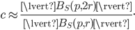
The expansion constant $c$ of a set $S$ is the smallest scalar $c \geq 2$ such that
$$\lvert B_S(p, 2r) \rvert \leq c B_S(p, r)$$
for all $p$, $r$. We will demonstrate that the expansion constant can be large and sensitive to changes in $S$.

Let $V = \mathbb{R}$ and let
$$S = \{ 2^i: i = 0, 1, 2, \dotsc, n \}$$
for some integer $n > 1$. In this case, $c = n$ because $\lvert B_S(2^n, 2^{n-1} - 0.5) \rvert = 1$ and $\lvert B_S(2^n, 2^n - 1) \rvert = n$ and this is obviously the worst case. Moreover, $c$ can be sensitive to changes of $S$, e.g., consider set $S$ whose points are evenly distributed on the surface of a unit hypersphere, and let $q \neq 0$ be a point arbitrarily close to the origin. The expansion constant of the set $S \cup \{0\}$ is $\lvert S \rvert + 1$ whereas the expansion constant of the set $S \cup \{ 0, q \}$ is $1/2 (\lvert S \rvert + 1)$ (this example was taken from the thesis Improving Dual-Tree Algorithms). With these bounds in mind and assuming the worst-case bounds on the cover tree algorithms are tight, we have to  concede that these algorithms may require $\mathcal{O}(n^6)$ operations or worse. Even if the points are regularly spaced, the performance bounds may be bad. Consider a set $S$ forming a $d$-dimensional hypercubic honeycomb, i.e., with $d=2$ this is a regular square tiling. In this case, the expansion constant $c$ is  proportional to $2^d$. Note that the expansion constant $c$ depends on the dimension of the subspace spanned by the points of $q \in S$ and not on the dimension of the space containing these points.

Nevertheless, cover trees are used in practice because real-world data sets often have small expansion constants. The expansion constant is related to the doubling dimension of a metric space (given a ball $B$ with unit radius in a $d$-dimensional metric space $V$, the doubling dimension of $V$ is the smallest number of balls with radius $r = 0.5$ needed to cover $B$).

Implementing Cover Trees

In a cover tree, given a point $p$ on level $i$, there is a node for $p$ on all levels $i, i-1, i-2, \dotso$ which raises the question how we can efficiently represent cover trees on a computer. Furthermore, we need to know if the number of levels in the cover tree can represented with standard integer types.

Given a point $p$ that occurs on multiple levels in the tree, we can either

• coalesce all nodes corresponding to $p$ and store the children in an associtive array whose values are child nodes and levels as keys, or
• we create one node corresponding to $p$ on each level whenever there are children, storing the level of the node as well as its children.

The memory consumption for the former representation can be calculated as follows: every cover tree node needs to store the corresponding point and the associative array. If the associative array is a binary tree, then for every level $i$, there is one binary tree node with

• a list of children of the cover tree node at level $i$,
• a pointer to its left child,
• a pointer to its right child, and
• a pointer to the parent binary tree node so that we can implement iterators (this is how std::map nodes in the GCC C++ standard library are implemented).

Hence, for every level $i$ in the binary tree, we need to store at least four references and the level. The other representation must store the level, a reference to the corresponding point, and a reference to the list of children of this cover tree node so this representation is more economic with respect to the memory consumption. There is no difference in the complexity of nearest-neighbor searches because for an efficient nearest-neighbor search, we have to search the cover tree top down starting at the highest level.

A metric maps its input to non-negative real values. On a computer (in finite precision arithmetic) there are bounds on the range of values that can be represented and we will elaborate on this fact using numbers in the IEEE-754 double-precision floating-point format as an example. An IEEE-754 float is a number $\pm m \cdot 2^{(e-b)}$, where $m$ is called the mantissa (or significand), $e$ is called the exponent, and $b$ is a fixed number called bias. The sign bit of a double-precision float is represented with one bit, the exponent occupies 11 bits, the mantissa 52 bits, and the bias is $b = 1024$. The limited size of these two fields immediately bounds the number the quantities that can be represented and in fact, the largest finite double-precision float value is approximately $2^{1024}$ and the smallest positive value is $2^{-1074}$. Consequently, we will never need have more than $1024 + 1074 = 2098$ levels in a cover tree when using double-precision floats irrespective of the number of points stored in the tree. Thus, the levels can be represented with 16bit integers.

Existing Implementations

The authors of the original cover tree paper Cover Trees for Nearest Neighbors made their C and C++ implementations available on the website http://hunch.net/~jl/projects/cover_tree/cover_tree.html. The first author of the paper Faster Cover Trees made the Haskell implementation of a nearest ancestor cover tree used for this paper available on GitHub. The C++ implementation by Manzil Zaheer features $k$-nearest neighbor search, range search, and parallel construction based on C++ concurrency features (GitHub). The C++ implementation by David Crane can be found in his repository on GitHub. Note that the worst-case complexity of node removal is linear in this implementation because of a conspicuous linear vector search. The most well maintained implementation of a cover tree can probably be found in the MLPACK library (also C++). I implemented a nearest ancestor cover tree in C++14 which takes longer to construct but has superior performance during nearest neighbor searches. The code can be found in my git repository.

Numerical Experiments

The worst-case complexity bounds of common cover tree operations, e.g., construction and querying, contain terms $c^6$ or $c^12$, where $c$ is the expansion constant. In this section, I will measure the effect of the expansion constant on the run-time of batch construction and nearest-neighbor search on a synthetic data set.

For the experiment, I implemented a nearest ancestor cover tree described in Faster Cover Trees in C++14 with batch construction, nearest-neighbor search (single-tree algorithm), and without associative arrays. The first point in the data set is chosen as the root of the cover tree and on every level of the cover tree, the construction algorithm attempts to select the points farthest away from the root as children.

The data consists of random points in $d$-dimensional space with uniformly distributed entries in the interval $[-1, +1)$, i.e., we use random points inside of a hypercube. The reference set (the cover tree) contains $n = 10^4$ points and we performed nearest-neighbor searches for $m = 10^3$ random points. The experiments are conducted using the Manhattan, the Euclidean, and the Chebychev metric and the measurements were repeated 25 times for dimensions $d = 10, 12, 14, \dotsc, 20$.

We do not attempt to measure the expansion constant for every set of points. Instead, we approximate the expansion constant from the dimension $d$. Let $d_p(\cdot, \cdot)$, $p = 1, 2, \infty$, be a metric, where

• $d_1(\cdot, \cdot)$ is the Manhattan metric,
• $d_2(\cdot, \cdot)$ is the Euclidean metric, and
• $d_{\infty}(\cdot, \cdot)$ is the Chebychev metric,

and let $B_p(d, r)$ be the ball centered at the origin with radius $r$:
$$B_p(d, r) := \{ p \in \mathbb{R}^d: d_p(0, p) \leq r \}.$$
The expansion constant $c$ of a set $S$ was defined as the smallest scalar $c \geq 2$ such that
$$\lvert B_S(p, 2r) \rvert \leq c \lvert B_S(p, r) \rvert$$
for all $p \in \mathbb{R}^d$, $r > 0$. We will now simplify both sides of the inequality.

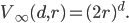
In this experiment, all entries of the points are uniformly distributed around the origin and using the assumption that $n$ and $r$ are sufficiently large, $B_S(p, r)$ will be approximately constant everywhere in the hypercube containing the points:
$$c \approx \frac{\lvert B_S(p, 2r) \rvert}{\lvert B_S(p, r) \rvert}.$$
Using the uniform distribution property again, we can set $p = 0$ without loss of generality. Likewise, since $\lvert B_S(0, r) \rvert$ is approximately constant, the fraction above will be close to the ratio of the volumes of the balls $B_p(d, 2r)$ and $B_p(d, r)$. $B_1(\cdot, \cdot)$ is called a cross-polytope and its volume can be computed with
$$V_1(d, r) = \frac{(2r)^d}{d!}.$$
The volume of the $d$-ball in Euclidean space $B_2(\cdot, \cdot)$ is
$$V_2(d, r) = \frac{\pi^{d/2}}{\Gamma(d/2+1)} r^d,$$
where $\Gamma$ is the gamma function. Finally, $B_{\infty}(d, r)$ is a hypercube with volume
$$V_{\infty}(d, r) = (2r)^d.$$
Using our assumptions, it holds that
$$c \approx \frac{V_p(d, 2r)}{V_p(d, r)} = 2^d, \, p = 1, 2, \infty.$$
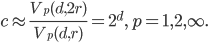
Consequently, the worst-case bounds are $2^{6d} n \log n$ for construction and $2^{12d} \log n$ for nearest-neighbor searches in cover trees with this data set.

In the plots, $p=1$ indicates the Manhattan, $p=2$ the Euclidean, and $p=\infty$ the Chebychev metric with the markers corresponding to the shape of the Ball $B_p(2, 1)$.

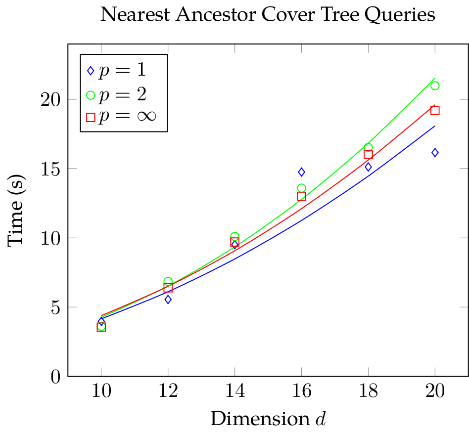
The figures below show mean and standard deviation for construction and query phase. The construction time of the cover tree is strongly dependent on the used metric: cover tree construction using the Chebychev metric takes considerably more time than with the other norms; construction with the Manhattan metric is slightly faster than with the Euclidean metric. Observe that there is a large variation in the construction time when employing the Euclidean metric and this effect becomes more pronounced the higher the dimension $d$. Also, considering the small standard deviation in the data, the construction time slightly jumps at $d=20$ for the Manhattan norm. In the query time plot, we can see that the results are mostly independent of the metric at hand. What is more, the variance of the query time is without exception small in comparison to the mean. Nevertheless, there is a conspicuous bend at $d=16$ when using the Manhattan metric. This bend is unlikely to be a random variation because we repeated the measurements 25 times and the variance is small.

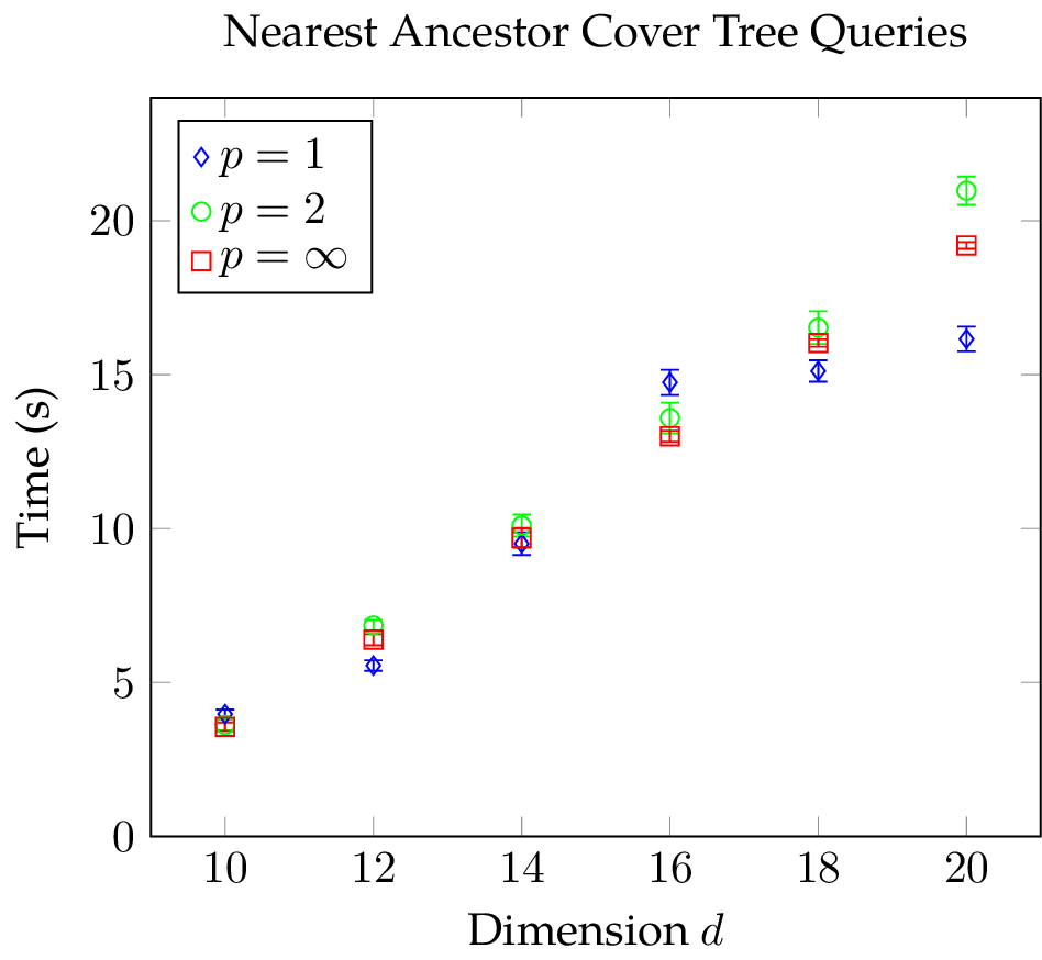
With our measurements we want to determine how the expansion constant influences construction and query time and according to the estimates above, we ought to see an exponential growth in operations. To determine if the data points could have been generated by an exponential function, one can plot the data with a logarithmic scaling along the vertical axis. Then, exponential functions will appear linear and polynomials sub-linear. In the figures below, we added an exponential function for comparison and it seems that the construction time does indeed grow exponentially with the dimension $d$ irrespective of the metric at hand while the query time does not increase exponentially with the dimension.

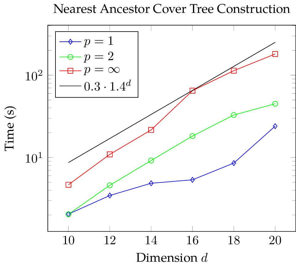
Seeing the logarithmic plots, I attempted to fit an exponential function $C \cdot b^d$, $C, b > 0$, to the construction time data. The fitted exponential did not approximate the data of the Euclidean and Manhattan metric well even when considering the standard deviation. However, the fit for the Chebychev metric was very good. In the face of these results, I decided to fit a monomial $C' d^e$, $C', e > 0$, to both construction and query time data and the results can be seen below. Except for the Manhattan metric data, the fit is very good.

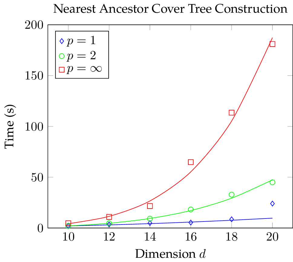
The value of the constants are for construction:

• $p=1$: $C' = 1.05 \cdot 10^{-2}$, $e = 2.28$,
• $p=2$: $C' = 5.74 \cdot 10^{-5}$, $e = 4.55$,
• $p = \infty$: $C' = 1.42 \cdot 10^{-5}$, $e = 5.47$.

For nearest-neighbor searches, the constants are

• $p=1$: $C' = 3.11 \cdot 10^{-2}$, $e = 2.12$,
• $p=2$: $C' = 1.95 \cdot 10^{-2}$, $e = 2.34$,
• $p = \infty$: $C' = 3.03 \cdot 10^{-2}$, $e = 2.16$.

In conclusion, for our test data the construction time of a nearest ancestor cover tree is strongly dependent on the metric at the hand and the dimension of the underlying space whereas the query time is mostly indepedent of the metric and a function of the square of the dimension $d$. The jumps in the data of the Manhattan metric and the increase in variation in the construction time when using the Euclidean metric highlight that there must be non-trivial interactions between dimension, metric, and the cover tree implementation.

Originally, we asked how the expansion constant $c$ impacts the run-time of cover tree operations and determined that we can approximate $c$ by calculating $c \approx 2^d$. Thus, the run-time $t$ of construction and nearest-neighbor search seems to be proportional to $\log c$ because $d \approx \log_2 c$ and $\log d^e = e \log d$.

Conclusion

We introduced cover trees, discussed their advantages as well as their unique theoretical properties. We elaborated on the complexity of cover tree operations, the expansion constant, and implementation aspects. Finally, we conducted an experiment on a synthetic data set and found that the construction time is strongly dependent on the metric and the dimension $d$ of the underlying space while the time needed for nearest-neighbor search is almost independent of the metric. Most importantly, the complexity of operations seems to be polynomial in $d$ and proportional to the logarithm of the expansion constant. There are unexplained jumps in the measurements.