In this blog post, I present stiffness and mass matrix as well as eigenvalues and eigenvectors of the Laplace operator (Laplacian) on domains $(0, \ell)$, $(0, \ell_1) \times (0, \ell_2)$, and so on (hyperrectangles) with zero Dirichlet boundary conditions discretized with the finite difference method (FDM) and the finite element method (FEM) on equidistant grids. For the FDM discretization, we use the central differences scheme with the standard five-point stencil in 2D. For the FEM, the ansatz functions are the hat functions. The matrices, standard eigenvalue problems $A v = \sigma v$, and generalized eigenvalue problems $K w = \tau M w$ arising from the discretization lend themselves for test problems in numerical linear algebra because they are well-conditioned, not diagonal, and the matrix dimension can be increased arbitrarily.

Python code generating the matrices and their eigenpairs can be found in my git repository discrete-laplacian.

Introduction

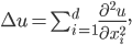
Let $d \in \mathbb{N} \setminus \{0\}$, let $u: \mathbb{R}^d \rightarrow \mathbb{R}$. The differential operator $\Delta$ is called Laplacian and it is the sum of the second derivatives of a function:
$$\Delta u = \sum_{i=1}^d \frac{\partial^2 u}{\partial x_i^2},$$
It is a well-researched differential operator in mathematics and for many domains, the exact eigenvalues $\lambda$ and eigenfunctions $u$ are known such that
$$-\Delta u = \lambda u.$$
In this blog post, I discuss the solutions of $-\Delta u = \lambda u$ on hyperrectangles $\Omega$ with the Dirichlet boundary condition
$$u = 0 \text{ on } \partial \Omega.$$

The combination of Laplace operator and the finite difference method (FDM) can be very well used in an introductory course on the numerical treatment of partial differential equations (PDEs) for the illustration of concepts such as discretization of PDEs, discretization error, the growth of the matrix condition number with finer grids, and sparse solvers.

In numerical linear algebra, the Laplace operator is appealing because the FDM discretization of the operator on a one-dimensional domain yields a standard eigenvalue problem $A v = \sigma v$ with a sparse, real symmetric positive-definite, tridiagonal Toeplitz matrix $A$ and known eigenpairs. For domains in higher dimensions, the matrices can be constructed with the aid of the Kronecker sum and consequently, the eigenpairs can be calculated in this case, too. With this knowledge, the Laplace operator makes for a good, easy test problem in numerical mathematics because we can distinguish between discretization errors and algebraic solution errors. Naturally, the Laplace operator can also be discretized with the finite element method (FEM) yielding a generalized eigenvalue problem $Kw = \tau Mw$ with sparse, real symmetric positive-definite matrices. Here, the eigenpairs are known, too, and furthermore, the eigenvectors are exact in the grid points (so-called superconvergence) providing us with another well-conditioned test problem.

I will present the solutions for the continuous case before I briefly introduce Kronecker products and Kronecker sums since these linear algebra operations are used to construct the matrices corresponding to higher dimensional domains. Finally, I discuss domain discretization and notation before giving closed expressions for the matrices and their eigenpairs created by FDM and FEM. In the end, there is an example demonstrating the use of the quantities $\ell_d$, $n_d$, and $h_d$.

Continuous Case

In 1D, the exact eigenpairs $(\lambda_i, u_i(x))$ of the Laplace operator on the domain $(0, \ell)$ are
$$\left(\frac{i^2}{\ell^2}\pi^2, \sin\frac{ix\pi}{\ell}\right), \, i = 1,2,\dotso.$$
In 2D, the exact eigenpairs $(\lambda_{ij}, u_{ij}(x))$ of the Laplace operator on the domain $(0, \ell_1) \times (0, \ell_2)$ are
$$\left( \left(\frac{i^2}{\ell_1^2} + \frac{j^2}{\ell_2^2}\right)\pi^2, \sin \frac{\pi i x_1}{\ell_1} \sin \frac{\pi j x_2}{\ell_2} \right), \, i, j = 1, 2, \dotso.$$
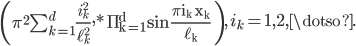
On a $d$-dimensional hyperrectangle, the eigenpairs are
$$\left( \pi^2 \sum_{k=1}^d \frac{i_k^2}{\ell_k^2}, \operatorname*{\Pi}_{k=1}^d \sin \frac{\pi i_k x_k}{\ell_k} \right), \, i_k=1,2,\dotso.$$
These solutions can be found, e.g., in the book Methods of Mathematical Physics, Vol. I, Chapter VI, §4.1.

Kronecker Products

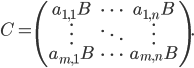
The matrices of the discretized Laplacian on higher dimensional domains can be constructed with Kronecker products. Given two matrices $A = [a_{ij}] \in \mathbb{R}^{m,n}$, $B \in \mathbb{R}^{k,\ell}$, the Kronecker product $C = A \otimes B$ is defined as follows:
$$C = \begin{pmatrix} a_{1,1} B & \cdots & a_{1,n} B \\ \vdots & \ddots & \vdots \\ a_{m,1} B & \cdots & a_{m,n} B \end{pmatrix}.$$
If $A$ and $B$ are square, then $C$ is square as well; let $(\lambda_i, v_i)$ be the eigenpairs of $A$ and let $(\mu_j, w_j)$ be the eigenpairs of $B$. Then the eigenpairs of $C$ are
$$(\lambda_i \mu_j, v_i \otimes w_j).$$
If $A$ and $B$ are real symmetric, then $C$ is also real symmetric. For square $A$ and $B$, the Kronecker sum of $A$ and $B$ is defined as
$$D = A \oplus B = I_k \otimes A + B \otimes I_m,$$
where $I_n$ is the $n \times n$ identity matrix. The eigenvalues of $D$ are
$$(\lambda_i + \mu_j, w_j \otimes v_i).$$
The Kronecker sum occurs during the construction of the 2D FDM matrix. See, e.g., Matrix Analysis for Scientists and Engineers by Alan J. Laub, Chapter 13, for more information on these operations.

Domain Discretization

For the 1D case along the $d$-th axis, we use $n_d+2$ points uniformly distributed over $(0, \ell_d)$, such that the step size is $h_d = \frac{\ell_d}{n_d+1}$. We use lexicographical ordering of points, e.g., in 2D let $u: \mathbb{R}^2 \rightarrow \mathbb{R}$ be an eigenfunction of the continuous problem, let $v \in \mathbb{R}^{n_1 n_2}$ be an eigenvector of the algebraic eigenvalue problem. Then $v_1$ is an approximation to $u(x_{1,1})$, $v_2$ approximates $u(x_{2,1})$, $v_{n_1+1}$ approximates $u(x_{1,2})$, and so on.

To obtain accurate approximations to the solutions of the continuous eigenvalue problem, the distance between adjacent grid points should always be constant. Thus, if the length of the 1D domain is doubled, the number of grid points should be doubled, too.

Notation

In the following sections, we need to deal with matrices arising from discretizations of the Laplace operator on 1D domains with different step sizes and their eigenpairs as well as discretizations of the Laplace operator on higher dimensional domains and their eigenpairs. $I$ denotes the identity matrix; its dimension can be gathered from the context.

Matrices $A$ denote the Laplacian discretized with the FDM, matrices $A^{(d)} \in \mathbb{R}^{n_d,n_d}$ denote the discrete Laplacian on 1D domains along the $d$-th axis, and matrices $A_d$ denote the the discrete Laplacian on a $d$-dimensional domain. The eigenpairs of $A^{(d)}$ are signified by $(\sigma_i^{(d)}, v_i^{(d)})$, $i = 1, 2, \dotsc, n_d$, $(\sigma_{i_1 i_2 \dotsb i_d}, v_{i_1 i_2 \dotsb i_d})$ are the eigenpairs of $A_d$.

Similarly, $K$ and $M$ are the stiffness and mass matrix, respectively, of the Laplace operator discretized with the finite element method. $K^{(d)}, M^{(d)} \in \mathbb{R}^{n_d,n_d}$ denote the discrete Laplacian on a one-dimensional domain along the $d$-th axis, and $K_d$, $M_d$ are the stiffness and mass matrix for the discrete Laplacian on a $d$-dimensional hyperrectangle. We speak of the solutions of $Kw = \tau M w$ or of eigenpairs of the matrix pencil $(K, M)$. The eigenpairs of $(K^{(d)}, M^{(d)})$ are denoted by $(\tau_i^{(d)}, w_i^{(d)})$, whereas $(\tau_{i_1 i_2 \dotsb i_d}, w_{i_1 i_2 \dotsb i_d})$ signify eigenpairs of $(K_d, M_d)$.

Finite Difference Method

In this section, we will construct the matrices of the discretized Laplace operator on a $d+1$-dimensional domain with the aid of the matrices for the $d$-dimensional and the one-dimensional case.

Let $e_i$ be the $i$-th unit vector. Let us consider the discretization along the $d$-th axis first. Let
$$(D^+ u)(x) = \frac{u(x + h_d e_d) - u(x)}{h_d}$$
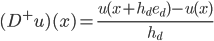
be the forward difference quotient, let
$$(D^- u)(x) = \frac{u(x) - u(x - h_d e_d)}{h_d},$$
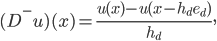
be the backward difference quotient. Then
$$\frac{\partial^2}{\partial x_d^2}(x) \approx (D^- D^+ u)(x) = \frac{u(x + h_d e_d) - 2 u(x) + u(x - h_d e_d)}{h_d^2}.$$
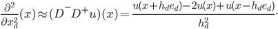
Consequently, the discrete Laplacian has the stencil
$$A^{(d)} = \frac{1}{h_d^2} \, \begin{bmatrix} -1 & 2 & -1 \end{bmatrix}$$
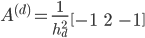
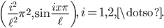
meaning $A^{(d)}$ is a real symmetric tridiagonal $n_d \times n_d$ matrix with the value 2 on the diagonal and -1 on the first sub- and superdiagonal. The eigenvalues of $A^{(d)}$ are
$$\sigma_i^{(d)} = \frac{2}{h_d^2} \left(1 - \cos \frac{\pi i}{n_d+1} \right), \, i=1,2,\dotsc,n_d,$$
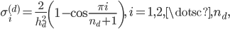
the entries of the eigenvector $v_i^{(d)}$ are
$$(v_i^{(d)})_k = \sin \frac{\pi k i}{n_d+1}, \, k=1,2,\dotsc,n_d .$$

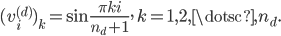
In 2D with lexicographic ordering of the variables, we have
$$A_2 = \frac{1}{h_1^2} \begin{bmatrix} 0&0&0 \\ -1&2&-1 \\ 0&0&0 \end{bmatrix} + \frac{1}{h_2^2} \begin{bmatrix} 0&-1&0 \\ 0&2&0 \\ 0&-1&0 \end{bmatrix}$$
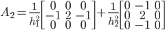
and this matrix can be constructed as follows:
$$A_2 = I \otimes A^{(1)} + A^{(2)} \otimes I.$$
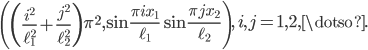
The eigenpairs can be derived directly from the properties of the Kronecker sum: the eigenvalues are
$$\sigma_{ij} = \sigma_j^{(2)} + \sigma_i^{(1)},$$
and the eigenvectors are
$$v_{ij} = v_j^{(2)} \otimes v_i^{(1)},$$
where $i = 1,2, \dotsc, n_1$, $j=1, 2, \dotsc, n_2$.

In higher dimensions, it holds that
$$A_{d+1} = I \otimes A_d + A^{(d+1)} \otimes I,$$
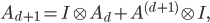
where
$$\sigma_{i_1 i_2 \dotsb i_{d+1}} = \sigma_{i_{d+1}}^{(d+1)} + \sigma_{i_1 i_2 \dotsb i_d}$$
are the eigenvalues and $$v_{i_1 i_2 \dotsb i_{d+1}} = v_{i_{d+1}}^{(d+1)} \otimes v_{i_1 i_2 \dotsb i_d}$$
are the eigenvectors, $i_{d+1} = 1, 2, \dotsc, n_{d+1}$.

Finite Element Method

Similarly to the finite differences method, we can construct the matrices of the discretized equation $-\Delta u = \lambda u$ recursively. We use hat functions as ansatz functions throughout this section.

The 1D stencil is
$$K^{(d)} = \frac{1}{h_d} \begin{bmatrix} -1 & 2 & -1 \end{bmatrix}$$
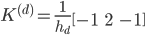
for the stiffness matrix and
$$M^{(d)} = \frac{h_d}{6} \begin{bmatrix} 1 & 4 & 1 \end{bmatrix}$$
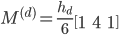
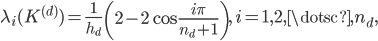
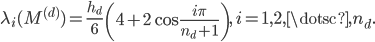
for the mass matrix. The generalized eigenvalues are
$$\tau_i^{(d)} = \frac{6}{h_d^2} \frac{1 - \cos \frac{i \pi}{n_d+1}}{2 + \cos \frac{i \pi}{n_d+1}}, \, i = 1, 2, \dotsc, n_d,$$
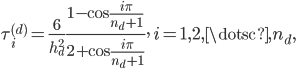
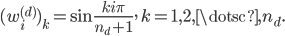
and the $k$-th entry of the eigenvector $w_i^{(d)}$ corresponding to $\tau_i^{(d)}$ is
$$(w_i^{(d)})_k = \sin \frac{k i \pi}{n_d+1}, \, k = 1, 2, \dotsc, n_d.$$
Observe that $w_i^{(d)}$ is not only an eigenvector of the matrix pencil $(K^{(d)}, M^{(d)})$ but also of the matrices $K^{(d)}$ and $M^{(d)}$ themselves. Thus, the eigenvalues of $K^{(d)}$ are
$$\lambda_i(K^{(d)}) = \frac{1}{h_d} \, \left(2 - 2 \cos \frac{i \pi}{n_d+1} \right), \, i=1,2,\dotsc,n_d,$$
whereas the eigenvalues of $M^{(d)}$ are
$$\lambda_i(M^{(d)}) = \frac{h_d}{6} \, \left(4 + 2 \cos \frac{i \pi}{n_d+1} \right), \, i=1,2,\dotsc,n_d.$$

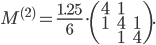
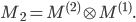
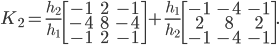
In 2D, the mass matrix stencil is
$$M_2 = \frac{h_1 h_2}{36} \begin{pmatrix} 1&4&1 \\ 4&16&4 \\ 1&4&1 \end{pmatrix}.$$
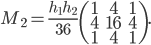
Judging by the coefficient $\frac{1}{36} h_1 h_2$ and the diagonal blocks, it must hold that
$$M_2 = M^{(2)} \otimes M^{(1)}.$$
The stiffness matrix stencil is
$$K_2 = \frac{h_2}{h_1} \begin{bmatrix} -1&2&-1 \\ -4&8&-4 \\ -1&2&-1 \end{bmatrix} + \frac{h_1}{h_2} \begin{bmatrix} -1&-4&-1 \\ 2&8&2 \\ -1&-4&-1 \end{bmatrix}.$$
Seeing the factors $h_1$ and $h_2$, the stiffness matrix cannot be the Kronecker product or the Kronecker sum of 1D stiffness matrices. However, observe that the 1D mass matrices $M^{(1)}$ and $M^{(2)}$ have coefficients $h_1$ and $h_2$, respectively, and indeed, the 2D stiffness matrix can be constructed with the aid of the 1D mass matrices:
$$K_2 = M^{(2)} \otimes K^{(1)} + K^{(2)} \otimes M^{(1)}.$$
Based on the properties of the Kronecker product and using the fact that mass and stiffness matrix have the same set of eigenvalues, $(K_2, M_2)$ has the eigenvalues
$$\tau_{ij} = \tau_j^{(2)} + \tau_i^{(1)}$$
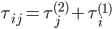
and eigenvectors
$$w_{ij} = w_j^{(2)} \otimes w_i^{(1)},$$
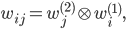
where $i = 1, 2, \dotsc, n_1$, $j = 1, 2, \dotsc, n_2$.

For the Laplacian on hyperrectangles in $d+1$-dimensional space, the stiffness matrix can be constructed by
$$K_{d+1} = M^{(d+1)} \otimes K_d + K^{(d+1)} \otimes M_d$$
the mass matrix can be constructed using
$$M_{d+1} = M^{(d+1)} \otimes M_d,$$
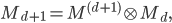
such that 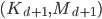$(K_{d+1}, M_{d+1})$ has eigenvalues
$$\tau_{i_1 i_2 \dotsb i_{d+1}} = \tau_{i_{d+1}}^{(d+1)} + \tau_{i_1 i_2 \dotsb i_d},$$
and eigenvectors
$$w_{i_1 i_2 \dotsb i_{d+1}} = w_{i_{d+1}}^{(d+1)} \otimes w_{i_1 i_2 \dotsb i_d},$$
where $i_{d+1} = 1, 2, \dotsc, n_{d+1}$.

Example

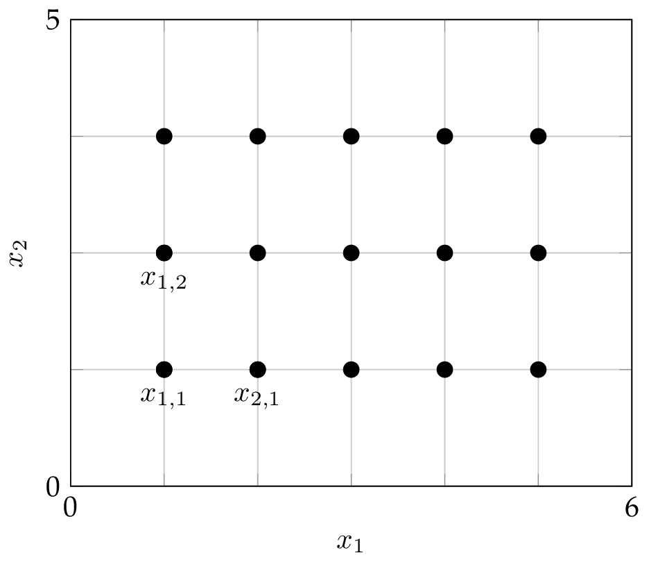
Now I will present the matrices of the discrete Laplacian on the domain $(0, 6) \times (0, 5)$. The figure below shows the domain and the grid used for discretization: there are five interior grid points along the first axis, three interior points along the second axis, and the interior grid points are highlighted as black circles. Thus, $\ell_1 = 6$, $\ell_2 = 5$, $n_1 = 5$, $n_2 = 3$, the step size $h_1 = 1$, and $h_2 = 1.25$. In 2D, an eigenvector $v$ of the algebraic eigenvalue problem will possess entries $v_i$, $i = 1, 2, \dotsc, 15$, such that $v_1 \approx u(x_{1,1})$, $v_2 \approx u(x_{2,1})$, $\dotsc$, $v_5 \approx u(x_{5,1})$, $v_6 \approx u(x_{1,2})$, $\dotsc$, $v_{15} \approx u(x_{5,3})$ because of the lexicographic ordering.

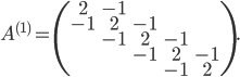
In the first dimension, the Laplacian discretized with the FDM has the following matrix:
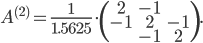
$$A^{(1)} = \begin{pmatrix} 2&-1 \\ -1&2&-1 \\ &-1&2&-1 \\ &&-1&2&-1 \\ &&&-1&2 \end{pmatrix}.$$ Along the second axis, we have
$$A^{(2)} = \frac{1}{1.5625} \cdot \begin{pmatrix} 2&-1 \\ -1&2&-1 \\ &-1&2 \end{pmatrix}.$$

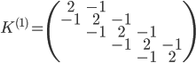
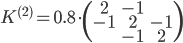
With the FEM, the stiffness matrix is
$$K^{(1)} = \begin{pmatrix} 2&-1 \\ -1&2&-1 \\ &-1&2&-1 \\ &&-1&2&-1 \\ &&&-1&2 \end{pmatrix}$$
and the mass matrix is
$$M^{(1)} = \frac{1}{6} \cdot \begin{pmatrix} 4&1 \\ 1&4&1 \\ &1&4&1 \\ &&1&4&1 \\ &&&1&4 \end{pmatrix}$$
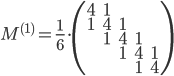
along the first axis. The matrices corresponding to the second dimension are
$$K^{(2)} = 0.8 \cdot \begin{pmatrix} 2&-1 \\ -1&2&-1 \\ &-1&2 \end{pmatrix}$$
and
$$M^{(2)} = \frac{1.25}{6} \cdot \begin{pmatrix} 4&1 \\ 1&4&1 \\ &1&4 \end{pmatrix}.$$