Given a linear algebra problem and an approximate solution, can we say something about the quality of the given approximate solution without knowing an exact solution?

In this post, let $x$ denote the problem data, let $y$ denote an exact solution, let $\widetilde{y}$ be an approximate solution, and let $f$ be a mapping such that $y = f(x)$. Moreover, let $\Delta x = \widetilde{x} - x$, where $\widetilde{x}$ is given in the next paragraph. $\lVert \cdot \rVert$ denotes a norm.

Bounding the Error

Can we say something about the forward error $\lVert \widetilde{y} - y \rVert$ without calculating $y$? The answer is yes, we can say something about the quality of the approximate solution by computing the backward error $\eta(x, \widetilde{y})$. It gives us the smallest distance between $x$ and some $\widetilde{x}$ such that $\widetilde{y} = f(\widetilde{x})$, i.e., the backward error is
$$\eta'(x, \widetilde{y}) := \min \{\lVert x-\widetilde{x}\rVert: f(\widetilde{x})=\widetilde{y} \}.$$
In conjunction with a Taylor series expansion of $f$ at  $x$ we can bound the forward error from above. Cutting  off the series expansion after the first-order term gives
$$\widetilde{y} = f(x + \Delta x) \approx f(x) + Df(x) \Delta x,$$
where $Df(x)$ signifies the Jacobian of $f$ at $x$. Substituting $\widetilde{y}$ into the definition of the forward error yields
$$\lVert \widetilde{y} - y \rVert \approx \lVert f(x) + Df(x) \Delta x - y \rVert = \lVert Df(x) \Delta x \rVert \leq \lVert Df(x) \rVert \lVert \Delta x \rVert,$$
where we used $y = f(x)$. Defining the condition number
$$\kappa'(x) := \lVert Df(x) \rVert$$
gives

forward error $\leq$ condition number $\times$ backward error.

Depending on its norm, the condition number can have the effect of a magnifier for errors. Note the condition number is problem dependent, i.e., on $f$ and $x$,  but independent of the approximate solution  $\widetilde{y}$ at hand. Consequently, for problems with large condition numbers we cannot expect (in general) a small forward error even if the backward error is tiny. Such problems are called ill-conditioned. Note that for consistency, condition number and backward error must use the same norm.

Bounding the Relative Error

Above, we defined absolute measures, i.e., the absolute forward error, the absolute condition number, and the  absolute backward error. These measures are not scale invariant and this makes it hard for us to determine when an error can be considered small. We can solve this  problem by using relative measures:

• the relative forward error $\frac{\lVert \widetilde{y}-y \rVert}{\lVert y \rVert}$,
• the relative backward error $\eta(x, \widetilde{y}) := \frac{1}{\lVert x \rVert} \eta'(x,\widetilde{y})$, and
• the relative condition number $\kappa(x) := \frac{\lVert x \rVert}{\lVert f(x) \rVert} \lVert Df(x) \rVert$.

For the relative backward error, it holds that
$$0 \leq \eta(x, \widetilde{y}) \leq 1,$$
where a value close to zero implies a good approximate  solution and a value close to one means that  $\widetilde{y}$ is the solution for a completely different problem. Furthermore, in finite precision arithmetic, i.e, on a computer, we can specify a value $\mathbf{u}$ such that every approximate solution with $\eta(x, \widetilde{y}) \leq \mathbf{u}$ can be considered accurate with respect to finite precision arithmetic. Let $a$ be the smallest, positive number without underflow, let $b$ be the largest finite number in finite precision arithmetic, f.e., with IEEE double precision floating point arithmetic,
$$a = 2^{-1022} \approx 2.225 \cdot 10^{-308}$$
and
$$b = 2 (1 - 2^{53}) \cdot 2^{1023} \approx 1.798 \cdot 10^{308},$$
let $r \in [a, b]$. Then for the floating point number  $\widetilde{r}$ closest to $r$, it holds that
$$\widetilde{r} = r (1 + \delta), \lvert \delta \rvert < \mathbf{u},$$
where $\mathbf{u}$ is called unit round-off. This is a relative backward error bound which is more obvious if we rewrite the equation as
$$\frac{\lvert \widetilde{r} - r \rvert}{\lvert r \rvert} < \mathbf{u}.$$
(It is simultaneously a forward error because the condition number is one.) If we cannot expect to represent a single number with a backward error less than $\mathbf{u}$, then we cannot expect to solve any problem with a backward error smaller than $\mathbf{u}$ either. Consequently, if the relative backward error is less than $\mathbf{u}$, we found a solution that can be considered as close as possible to an exact solution in finite precision arithmetic. Note the unit round-off $\mathbf{u}$ is related to the machine epsilon $\varepsilon$ by $\varepsilon = 2 \mathbf{u}$. Also, with IEEE double precision floats, $\mathbf{u} = 2^{-53} \approx 1.11 \cdot 10^{-16}$.

In general, it is undesirable to directly bound the forward error because bounding the forward error gives weaker bounds on the backward error than the other way around. What is more, for ill-conditioned problems the backward error remains a reliable termination criterion termination while the forward error does not. Thus, our measure for solution quality will be the backward error.

The Backward Error in Practice

Using relative backward errors, we can assess the accuracy of an approximate solution without the need for exact solutions. To put the icing on the cake, for many linear algebra problems there are closed-form expressions for the relative backward error using common and intuitive norms. That is, we can evaluate the quality of a solution by calculating matrix-vector products and vector norms irrespective of the level of difficuly of the problem. For example, for a system of linear equations $A x = b$, we have
$$\eta(A, b, \widetilde{x}) = \frac{\lVert b - A\widetilde{x}\rVert}{\lVert A \rVert \lVert \widetilde{x} \rVert + \lVert b \rVert}.$$

Example: A System of Linear Equations

Consider the SLE $A x = b$, where
$$A = \begin{pmatrix} -5 & 15 \\ 2 & 10 \end{pmatrix}, x = \begin{pmatrix} 5 \\ 1 \end{pmatrix}, b = \begin{pmatrix} -10 \\ 20 \end{pmatrix},$$
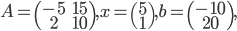
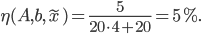
let $\widetilde{x} = (4, 1)^T$ be an approximate solution. Let $\lVert\cdot\rVert$ be the maximum norm. Then the backward error is
$$\eta(A, b, \widetilde{x}) = \frac{5}{20 \cdot 4 + 20} = 5\%.$$

The Backward Error in Practice (cont'd)

For a more complicated generalized eigenvalue problem $K x = \lambda M x$, $K, M \in \mathbb{C}^{n,n}$, the relative backward error of an eigenpair $(\widetilde{\lambda}, \widetilde{x})$ can be calculated with
$$\eta(K, M, \widetilde{\lambda}, \widetilde{x}) = \frac{1}{\lVert x \rVert} \frac{\lVert K \widetilde{x} - \widetilde{\lambda} M \widetilde{x} \rVert}{\lVert K \rVert + \lvert \widetilde{\lambda} \rvert \lVert M \rVert}.$$
Moreover, we can often take problem structure into account which gives us structured backward errors and condition numbers.

Example: Problem Structure and Backward Error

Consider the standard eigenvalue problem $A x = \lambda x$, where
$$A = \begin{pmatrix} 0 & +1 \\ -1 & 0 \end{pmatrix}$$
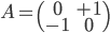
is real skew-symmetric and has the eigenvalues $\lambda_1 = +i, \lambda_2 = -i$. In this example, we measure the distance between two matrices using the Frobenius norm $\lVert \cdot \rVert_F$. Consider the approximate eigenvalue $\widetilde{\lambda} = 0$, then
$$\widetilde{A} = \begin{pmatrix} 0 & 1 \\ 0 & 0 \end{pmatrix}$$
is a matrix closest to $A$ possessing the eigenvalue $\widetilde{\lambda}$. Consequently,
$$\eta(A, \widetilde{\lambda}) = \lVert \widetilde{A} - A \rVert_F = 1.$$
The result is unsatisfying insofar as $\widetilde{A}$ is not skew-symmetric so let us restrict the set of perturbations to the set of real skew-symmetric matrices and let $\eta^S(\cdot, \cdot)$ denote the corresponding structured backward error. Then $\widetilde{A}_S = 0$ is the matrix closest to $A$ possessing the  eigenvalue $\widetilde{\lambda} = 0$ and the structured backward error is $\eta^S(A, \widetilde{\lambda}) = \sqrt{2}$.

The Condition Number in Practice

For the relative condition number, we have to make a slight concession: we cannot evaluate it exactly because the exact solution occurs in the denominator. For  example, the condition number for linear systems $A x = b$ is
$$\kappa(A, b) = \frac{\lVert A^{-1} \rVert \lVert b \rVert}{\lVert x \rVert} + \lVert A \rVert \lVert A^{-1} \rVert$$
with the solution $x$ appearing in the first term. In practice, this fact is neglected and the approximate solution $\widetilde{x}$ is used. Moreover, we might need to compute matrix norms. This is a simple task for the row sum and the column sum norm but expensive or downright impossible for the spectral norm. In the worst case, we need the norm of a matrix inverse. Luckily, we can estimate this norm for the row sum and the column sum norm.

Conclusion

In linear algebra we can evaluate the quality of an approximate solution by computing its backward error and the condition number of the problem. In finite precision arithmetic, the backward error is also the method of choice for robust termination criteria.

A comprehensive book about backward errors and condition numbers for many problems in linear algebra is Nicholas J. Higham's Accuracy and Stability of Numerical Algorithms. Unfortunately, it does not discuss eigenvalue problems. Standard eigenvalue problems are discussed in Stewart and Sun's Matrix Perturbation Theory, Higham and Higham's paper Structured Backward Error and Condition of Generalized Eigenvalue Problems deals with generalized eigenvalue problems. Adhikari, Alam, and Kressner present closed-form expressions for the backward error and the condition number for  structured polynomial eigenvalue problems in their papers On backward errors of structured polynomial eigenproblems solved by structure preserving linearizations (preprint) and Structured eigenvalue condition numbers and linearizations for matrix polynomials (preprint, verbatim capitalization).

Throughout this post, we used normwise error bounds but for certain problems, we can bound the error for every component of the data. Accordingly, this concept is called the componentwise error in contrast to the normwise error. In the literature, the letters $\eta$ and $\kappa$ are used to signify both relative and absolute measures because the definition of the backward error is slightly more flexible than in this post; see, f.e., the theorem of Rigal and Gaches in Higham's book "Accuracy and Stability of Numerical Algorithms".